JAXsim Showcase: Parallel Simulation of a free-falling body

First, we install the necessary packages and import them.

# @title Imports and setup
import sys

IS_COLAB = "google.colab" in sys.modules

# Install JAX and Gazebo
if IS_COLAB:
    !{sys.executable} -m pip install -qU jaxsim
    !apt install -qq lsb-release wget gnupg
    !wget https://packages.osrfoundation.org/gazebo.gpg -O /usr/share/keyrings/pkgs-osrf-archive-keyring.gpg
    !echo "deb [arch=$(dpkg --print-architecture) signed-by=/usr/share/keyrings/pkgs-osrf-archive-keyring.gpg] http://packages.osrfoundation.org/gazebo/ubuntu-stable $(lsb_release -cs) main" | sudo tee /etc/apt/sources.list.d/gazebo-stable.list > /dev/null
    !apt -qq update
    !apt install -qq --no-install-recommends libsdformat13 gz-tools2

# Set environment variable to avoid GPU out of memory errors
%env XLA_PYTHON_CLIENT_MEM_PREALLOCATE=false

import time

import jax
import jax.numpy as jnp
import rod
from rod.builder.primitives import SphereBuilder

from jaxsim import logging

logging.set_logging_level(logging.LoggingLevel.INFO)
logging.info(f"Running on {jax.devices()}")

env: XLA_PYTHON_CLIENT_MEM_PREALLOCATE=false

jaxsim[3488] INFO Running on [CpuDevice(id=0)]

We will use a simple sphere model to simulate a free-falling body. The spheres set will be composed of 9 spheres, each with a different position. The spheres will be simulated in parallel, and the simulation will be run for 3000 steps corresponding to 3 seconds of simulation.

Note: Parallel simulations are independent of each other, the different position is imposed only to show the parallelization visually.

# @title Create a sphere model
model_sdf_string = rod.Sdf(
    version="1.7",
    model=SphereBuilder(radius=0.10, mass=1.0, name="sphere")
    .build_model()
    .add_link()
    .add_inertial()
    .add_visual()
    .add_collision()
    .build(),
).serialize(pretty=True)

JAXsim offers a simple functional API in order to interact in a memory-efficient way with the simulation. Four main elements are used to define a simulation:

• model: an object that defines the dynamics of the system.

• data: an object that contains the state of the system.

• integrator: an object that defines the integration method.

• integrator_state: an object that contains the state of the integrator.

import jaxsim.api as js
from jaxsim import integrators

dt = 0.001
integration_time = 1.5  # seconds

model = js.model.JaxSimModel.build_from_model_description(
    model_description=model_sdf_string
)
data = js.data.JaxSimModelData.build(model=model)
integrator = integrators.fixed_step.RungeKutta4SO3.build(
    dynamics=js.ode.wrap_system_dynamics_for_integration(
        model=model,
        data=data,
        system_dynamics=js.ode.system_dynamics,
    ),
)
integrator_state = integrator.init(x0=data.state, t0=0.0, dt=dt)

jaxsim[3488] INFO The kinematic graph doesn't need to be reduced

It is possible to automatically choose a good set of parameters for the terrain.

By default, in JaxSim a sphere primitive has 250 collision points. This can be modified by setting the JAXSIM_COLLISION_SPHERE_POINTS environment variable.

Given that at its steady-state the sphere will act on two or three points, we can estimate the ground parameters by explicitly setting the number of active points to these values.

Eventually, you can specify the maximum penetration depth of the sphere into the terrain by passing max_penetraion to the estimate_good_soft_contacts_parameters function.

data = data.replace(
    contacts_params=js.contact.estimate_good_soft_contacts_parameters(
        model=model,
        number_of_active_collidable_points_steady_state=3,
        max_penetration=None,
    )
)

Let’s create a position vector for a 4x4 grid. Every sphere will be placed at a different height.

# Primary Calculations
envs_per_row = 4  # @slider(2, 10, 1)

env_spacing = 0.5
edge_len = env_spacing * (2 * envs_per_row - 1)


# Create Grid
def grid(edge_len, envs_per_row):
    edge = jnp.linspace(-edge_len, edge_len, envs_per_row)
    xx, yy = jnp.meshgrid(edge, edge)
    zz = 0.2 + 0.1 * (
        jnp.arange(envs_per_row**2) % envs_per_row
        + jnp.arange(envs_per_row**2) // envs_per_row
    )
    zz = zz.reshape(envs_per_row, envs_per_row)
    poses = jnp.stack([xx, yy, zz], axis=-1).reshape(envs_per_row**2, 3)
    return poses


logging.info(f"Simulating {envs_per_row**2} environments")
poses = grid(edge_len, envs_per_row)

jaxsim[3488] INFO Simulating 16 environments

In order to parallelize the simulation, we first need to define a function simulate for a single element of the batch.

# Define a function to simulate a single model instance
def simulate(
    data: js.data.JaxSimModelData, integrator_state: dict, pose: jnp.array
) -> tuple:
    # Set the base position to the initial pose
    data = data.reset_base_position(base_position=pose)

    # Create a list to store the base position over time
    x_t_i = []

    for _ in range(int(integration_time // dt)):
        data, integrator_state = js.model.step(
            dt=dt,
            model=model,
            data=data,
            integrator=integrator,
            integrator_state=integrator_state,
            joint_forces=None,
            link_forces=None,
        )
        x_t_i.append(data.base_position())

    return x_t_i

We will make use of jax.vmap to simulate multiple models in parallel. This is a very powerful feature of JAX that allows to write code that is very similar to the single-model case, but can be executed in parallel on multiple models. In order to do so, we need to first apply jax.vmap to the simulate function, and then call the resulting function with the batch of different poses as input.

Note that in our case we are vectorizing over the pose argument of the function simulate, this correspond to the value assigned to the in_axes parameter of jax.vmap:

in_axes=(None, None, 0) means that the first two arguments of simulate are not vectorized, while the third argument is vectorized over the zero-th dimension.

# Define a function to simulate multiple model instances
simulate_vectorized = jax.vmap(simulate, in_axes=(None, None, 0))

# Run and time the simulation
now = time.perf_counter()

x_t = simulate_vectorized(data, integrator_state, poses)

comp_time = time.perf_counter() - now

logging.info(
    f"Running simulation with {envs_per_row**2} models took {comp_time} seconds."
)
logging.info(
    f"This corresponds to an RTF (Real Time Factor) of {(envs_per_row**2 * integration_time / comp_time):.2f}"
)

jaxsim[3488] INFO Running simulation with 16 models took 38.96615235200079 seconds.

jaxsim[3488] INFO This corresponds to an RTF (Real Time Factor) of 0.62

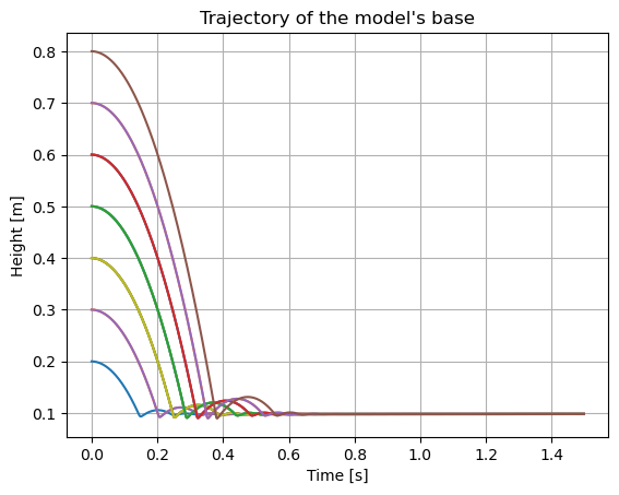
Now let’s extract the data from the simulation and plot it. We expect to see the height time series of each sphere starting from a different value.

import matplotlib.pyplot as plt
import numpy as np

plt.plot(np.arange(len(x_t)) * dt, np.array(x_t)[:, :, 2])
plt.grid(True)
plt.xlabel("Time [s]")
plt.ylabel("Height [m]")
plt.title("Trajectory of the model's base")
plt.show()